11. Radial and Axial Expansion and Contraction

ARMI natively supports linear expansion in both the radial and axial dimensions for pin-type reactors. These expansion types function independently of one another and each have their own set of underlying assumptions and use-cases. Radial expansion happens by default but there are several settings that control axial expansion:

• inputHeightsConsideredHot - Indicates whether blueprints heights have already been thermally expanded. If False, ARMI will expand components at BOL consistent with provided temperatures.

• assemFlagsToSkipAxialExpansion - Assemblies with a flag in this list will not be axially expanded.

• detailedAxialExpansion - Allow each assembly to expand independently. This will result in a non-uniform mesh.

If they happen, ARMI runs radial and axial expansion when objects are created from blueprints. That is, when the reactor is created from blueprints at BOL, these calculations are performed. But also at BOC if new assemblies are added to the core, then expansion will happen again when the assembly object is created from blueprints.

11.1. Thermal Expansion

ARMI treats thermal expansion as a linear phenomena using a standard linear expansion relationship,

(1)\[\frac{\Delta L}{L_0} = \alpha(T) \Delta T,\]

where, \(\Delta L\) and \(\Delta T\) are the change in length and temperature from the reference state, respectively, and \(\alpha\) is the thermal expansion coefficient relative to \(T_0\). Expanding and rearranging Equation (1), we can obtain an expression for the new length, \(L_1\),

(2)\[L_1 = L_0\left[1 + \alpha(T_1)\left(T_1 - T_0\right) \right].\]

Given Equation (1), we can create expressions for the change in length between our “hot” temperature (Equation (3))

(3)\[\begin{split}\begin{aligned} \frac{L_h - L_0}{L_0} &= \alpha(T_h)\left(T_h - T_0\right),\\ \frac{L_h}{L_0} &= 1 + \alpha(T_h)\left(T_h - T_0\right). \end{aligned}\end{split}\]

and “non-reference” temperature, \(T_c\) (Equation (4)),

(4)\[\begin{split}\begin{aligned} \frac{L_c - L_0}{L_0} &= \alpha(T_c)\left(T_c - T_0\right),\\ \frac{L_c}{L_0} &= 1 + \alpha(T_c)\left(T_c - T_0\right). \end{aligned}\end{split}\]

These are used within ARMI to enable thermal expansion and contraction with a temperature not equal to the reference temperature, \(T_0\). By taking the difference between Equation (3) and (4), we can obtain an expression relating the change in length, \(L_h - L_c\), to the reference length, \(L_0\),

(5)\[\begin{split}\begin{aligned} \frac{L_h - L_0}{L_0} - \frac{L_c - L_0}{L_0} &= \frac{L_h}{L_0} - 1 - \frac{L_c}{L_0} + 1, \\ &= \frac{L_h - L_c}{L_0}. \end{aligned}\end{split}\]

Using Equations (5) and (4), we can obtain an expression for the change in length, \(L_h - L_c\), relative to the non-reference temperature,

(6)\[\begin{split}\frac{L_h - L_c}{L_c} &= \frac{L_h - L_c}{L_0} \frac{L_0}{L_c}\\ &= \left( \frac{L_h}{L_0} - \frac{L_c}{L_0} \right) \left( 1 + \alpha(T_c)\left(T_c - T_0\right) \right)^{-1}.\end{split}\]

Using Equations (3) and (4), we can simplify Equation (6) to find,

(7)\[\frac{L_h - L_c}{L_c} = \frac{\alpha(T_h) \left(T_h - T_0\right) - \alpha(T_c)\left(T_c - T_0\right)}{1 + \alpha(T_c)\left(T_c - T_0\right)}.\]

Equation (7) is the expression used by ARMI in linearExpansionFactor.

Note

linearExpansionPercent returns \(\frac{L - L_0}{L_0}\) in %.

Given that thermal expansion (or contraction) of solid components must conserve mass throughout the system, the density of the component is adjusted as a function of temperature based on Equation (8), assuming isotropic thermal expansion.

(8)\[\rho(T_h) = \frac{\rho(T_0)}{\left(1 + \frac{\Delta L}{L_0}\right)^3} = \frac{\rho(T_0)}{\left(1 + \alpha_m (T_h) (T_h - T_0)\right)^3}\]

where, \(\rho(T_h)\) is the component density in \(\frac{kg}{m^3}\) at the given temperature \(T_h\), \(\rho(T_0)\) is the component density in \(\frac{kg}{m^3}\) at the reference temperature \(T_0\), and \(\alpha(T_h)\) is the mean coefficient of thermal expansion at the specified temperature \(T_h\) relative to the material’s reference temperature.

An update to mass densities is applied for all solid components given the assumption of isotropic thermal expansion. Here we assume the masses of non-solid components (e.g., fluids or gases) are allowed to change within the reactor core model based on changes to solid volume changes. For instance, if solids change volume due to temperature changes, there is a change in the amount of volume left for fluid components.

11.2. Implementation Discussion and Example of Radial and Axial Thermal Expansion

This section provides an example thermal expansion calculation for a simple cylindrical component from a reference temperature of 20°C to 1000°C with example material properties and dimensions as shown in the table below.

Example Component Properties for Thermal Expansion

Property	Example
Material	Steel
Radius	0.25 cm
Height	5.0 cm
Reference Temperature	20°C
Density	1.0 g/cc
Mean Coefficient Thermal Expansion	\(2\times 10^{-6}\) 1/°C

The figure below illustrates the thermal expansion phenomena in both the radial and axial directions.

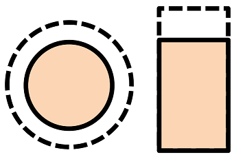
Illustration of radial and axial thermal expansion for a cylinder in ARMI.

Thermal expansion calculations are performed for each component in the ARMI reactor data model as component temperatures change. Since components are constrained within blocks, the height of components are determined by the height of their parent block. Equations (9) through (12) illustrate how the radius, height, volume, density, and mass are updated for a Component during thermal expansion, respectively.

Example Calculation of Radial and Axial Thermal Expansion for a Cylindrical Component

Component Temperature	20°C	1000°C
Radius	0.25 cm	0.251 cm
Height	5.0 cm	5.01 cm
Volume	0.982 cc	0.988 cc
Density	1.0 g/cc	0.994 g/cc
Mass	0.982 g	0.982 g

(9)\[ r(T_h) = 0.25 \left(1 + \left(2\times 10^{-6}(1000 − 20)\right)\right) = 0.251 cm\]

(10)\[ h(T_h) = 5.0 \left(1 + \left(2\times 10^{-6}(1000 − 20)\right)\right) = 5.01 cm\]

(11)\[ V(T_h) = \pi (0.251)^2 5.01 = 0.988 cm^3\]

(12)\[ \rho(T_h) = \frac{1.0}{\left(1 + 2\times 10^{-6}(1000 − 20)\right)^3} = 0.994 \frac{g}{cc}\]

(13)\[ m(T_h) = 0.994 \times 0.988 = 0.982 g\]

Radial thermal expansion occurs for each Component in a given Block. Mechanical contact between components is not accounted for, meaning that the radial expansion of one Component is independent from the radial expansion of the others. Solid components may be radially linked to gas/fluid components (i.e., sodium bond, helium) and the gas/fluid area is allowed to radially expand and contract with changes in Component temperature. It is worth noting that void components are allowed to have negative areas in cases where the expansion of two solid components overlap each other.

Axial thermal expansion occurs for each solid Component with a given Block. Axial mechanical contact between components is accounted for as the expansion or contraction of a Component affects the positions of components in mechanical contact in axially neighboring blocks. The logic for determining Component-to-Component mechanical contact is described in Section Component-to-Component Axial Linking. When two or more solid components exist within the Block, the change in Block height is driven by an axial expansion “target Component” (e.g., fuel). The logic for determining the axial expansion “target Component” is provided in Section Target Component Logic.

Figures Illustration of Components for Axial Thermal Expansion Process and Simplified Illustration of Axial Thermal Expansion Process for a Core Assembly provide illustrations of the axial thermal expansion process for an example core assembly. In this example there are four main block types defined: Shield, Fuel, Plenum, and Dummy.

Note

The “dummy” Block is necessary to maintain a consistent core-wide assembly height as this is a common necessity for physics solvers utilizing discrete-ordinates discretization methods.

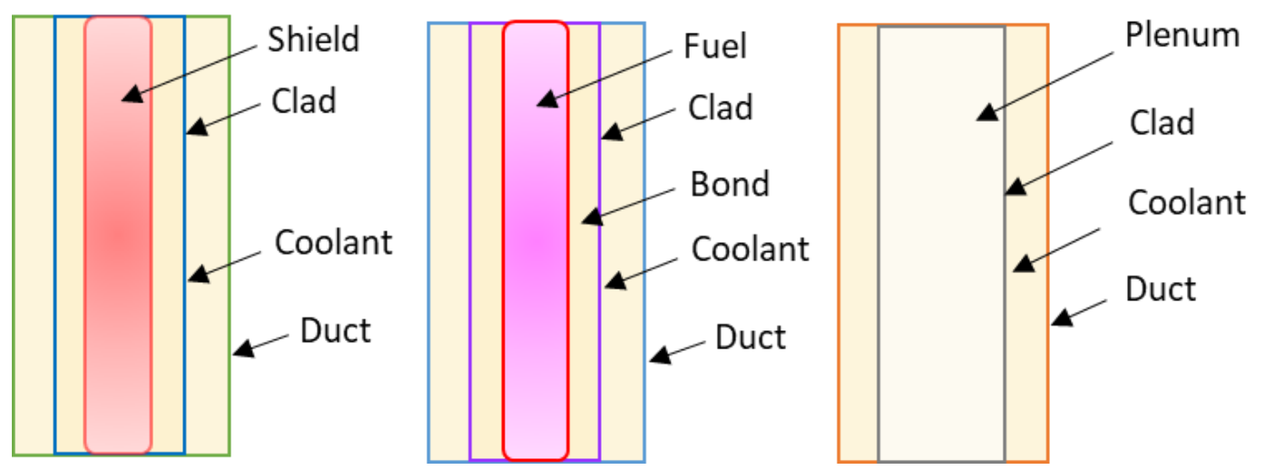
Illustration of Components for Axial Thermal Expansion Process

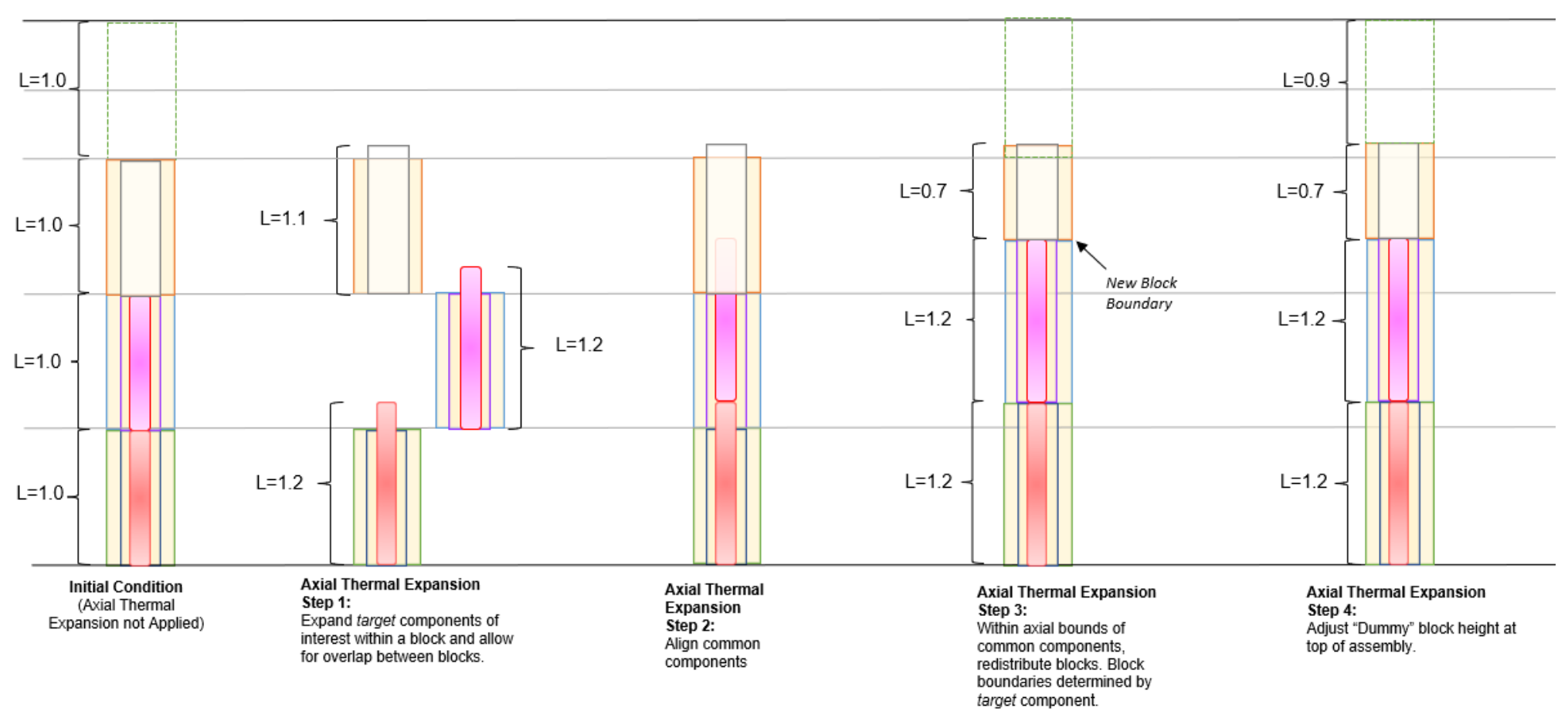
Simplified Illustration of Axial Thermal Expansion Process for a Core Assembly

The target components for each Block type are provided in the following table:

Example Assignment of Target Components within Blocks

Block	Target Component
Shield	Shield
Fuel	Fuel
Plenum	Clad
Dummy	N/A

The axial thermal expansion algorithm is applied in four steps:

1. Expand the axial dimensions of each solid Component within each block independently.

2. Align blocks axially such that axially-linked components have consistent alignments (e.g., overlapping radial dimensions).

3. Assign the Block lower and upper elevations to account for the thermal expansion of blocks below each Block.

   • Create new mesh lines (i.e., Block bounds) that track the target component.

4. Adjust the “dummy” Block located at the top of the assembly to maintain a consistent core-wide assembly height before and after axial thermal expansion is applied.

11.2.1. Component-to-Component Axial Linking

For components to be in mechanical contact, and therefore axially linked, they need to meet the following criteria:

1. The same Component class. E.g., both are basicShapes.Circle.

2. Both solid materials.

If those are met, then geometric overlap may be checked if the following are met:

1. The components are not components.UnshapedComponent

2. The components have the same multiplicity

3. Or, they share the same grid indices, as specified by a Block <grid> grids.locations.MultiIndexLocation.

Finally, geometric overlap is established if the biggest inner bounding diameter of the components is less than the smallest outer bounding diameter of the components.

11.2.1.1. Limitations

A current limitation of the axial linking logic is that multiple Components may not be linked to a single Component. E.g., consider the following:

1. A solid cylinder with an outer diameter of 1.0 cm.

2. Above, a solid cylinder wrapped with an annular cylinder (separate ARMI components) each with the following dimensions:

• Solid cylinder with an outer diameter of 0.5 cm.

• Annulus with inner diameter of 0.5 cm and outer diameter of 0.75 cm.

For the above example, in reality, the annulus wrapped pin (two separate ARMI components) would be affected by any changes in height from the solid cylinder. However, this set up is not allowed by the current implementation and will raise a RuntimeError.

A second limitation of the component linking implementation involves the Block grid based approach. When Block grids are used to specify a pin lattice, the Block-grid should be used throughout the Assembly definition; i.e., a mixture of the Block-grid and multiplicity assignment should not be used (and will likely produce unexpected results and may even fail). For example, in the following partial blueprint definition, in reality, each shield pin should be in mechanical contact with the fuel pins. However, since there is a mixture of mulitiplicity and Block-grid approaches, they are assumed to be not-linked. In order to ensure properly linking, block_fuel_axial_shield needs to be redefined with the Block-grid based approach.

axial shield: &block_fuel_axial_shield
  shield:
    shape: Circle
    material: HT9
    Tinput: 25.0
    Thot: 600.0
    id: 0.0
    mult: 169.0
    od: 0.86602

fuel multiPin: &block_fuel_multiPin
  grid name: twoPin
  fuel 1: &component_fuelmultiPin
    shape: Circle
    material: UZr
    Tinput: 25.0
    Thot: 600.0
    id: 0.0
    od: 0.86602
    latticeIDs: [1]
  fuel 2:
    <<: *component_fuelmultiPin
    latticeIDs: [2]

The following incorporates the fix for block_fuel_axial_shield and illustrates another potentially undesirable situation where unexpected results or runtime failure may occur. Here a plenum block is added above the fuel and while it does utilize a Block-grid, clad will not be axially linked to either the fuel 1 or fuel 2 components below it. This is because the clad and fuel* components have different grids via their grid.spatialLocator values. As in the previous example, similar unexpected behavior would also occur if a multiplicity-based definition were used for clad.

axial shield multiPin: &block_fuel_multiPin_axial_shield
  grid name: twoPin
  shield 1: &component_shield_shield1
    shape: Circle
    material: HT9
    Tinput: 25.0
    Thot: 600.0
    id: 0.0
    od: 0.8
    latticeIDs: [1]
  shield 2:
    <<: *component_shield_shield1
    latticeIDs: [2]

fuel multiPin: &block_fuel_multiPin
  grid name: twoPin
  fuel 1: &component_fuelmultiPin
    shape: Circle
    material: UZr
    Tinput: 25.0
    Thot: 600.0
    id: 0.0
    od: 0.8
    latticeIDs: [1]
  fuel 2:
    <<: *component_fuelmultiPin
    latticeIDs: [2]

plenum 2pin: &block_plenum_multiPin
  grid name: twoPin
  clad:
    shape: Circle
    material: Void
    Tinput: 25.0
    Thot: 600.0
    id: 0.9
    od: 1.0
    latticeIDs: [1,2]

To resolve this potential issue, block_plenum_multiPin should be replaced with the following definition. See the multi pin fuel assembly definition within armi/tests/detailedAxialExpansion/refSmallReactorBase.yaml for a complete example.

plenum 2pin: &block_plenum_multiPin
grid name: twoPin
clad 1: &component_plenummultiPin_clad1
    shape: Circle
    material: Void
    Tinput: 25.0
    Thot: 600.0
    id: 0.9
    od: 1.0
    latticeIDs: [1]
clad 2:
  <<: *component_plenummultiPin_clad1
    latticeIDs: [2]

11.2.2. Target Component Logic

When two or more solid components exist within a Block, the overall height change of the Block is driven by an “axial expansion target component” (e.g., fuel). This Component may either be inferred from the flags prescribed in the blueprints or manually set using the axial expansion target component block blueprint attribute. The following logic is used to infer the target component:

1. Search Component flags for neutronically important components. These are defined in expansionData.TARGET_FLAGS_IN_PREFERRED_ORDER.

2. Compare the Block and Component flags. If a Block and Component contain the same flags, that Component is selected as the axial expansion target Component.

3. If a Block has flags.flags.PLENUM or flags.flags.ACLP, the flags.flags.CLAD Component is hard-coded to be the axial expansion target component. If one does not exist, an error is raised.

4. “Dummy Blocks” are intended to only contain fluid (generally coolant fluid), and do not contain solid components, and therefore do not have an axial expansion target component.

11.2.3. Mass Conservation

Due to the fact that all components within a Block are the same height, the conservation of mass post-axial expansion is not trivial. The axial expansion target component plays a critical role in the conservation of mass. For pinned-blocks, this is typically chosen to be the most neutronically important Component; e.g., in a fuel Block this is typically the fuel Component. Generally speaking, components which are not the axial expansion target will exhibit non-conservation on the Block-level as mass is redistributed across the axially- neighboring blocks; this is discussed in more detail in Section 11.2.3.1. However, the mass of all solid components are designed to be conserved at the assembly-level if the following are met for a given assembly design.

1. Axial continuity of like-objects. E.g., pins, clad, etc.

2. Components that may expand at different rates axially terminate in unique blocks

   • E.g., the clad extends above the termination of the fuel and the radial duct encasing an assembly extends past the termination of the clad.

3. The top-most Block must be a “dummy Block” containing fluid (typically coolant).

See armi.tests.detailedAxialExpansion for an example blueprint which satisfy the above requirements.

11.2.3.1. Block-Level Mass Redistribution

Figure Illustration of mass redistribution for axial expansion in ARMI. illustrates the mass redistribution process for axial expansion in ARMI given a uniform axial expansion of 10% for fuel components.

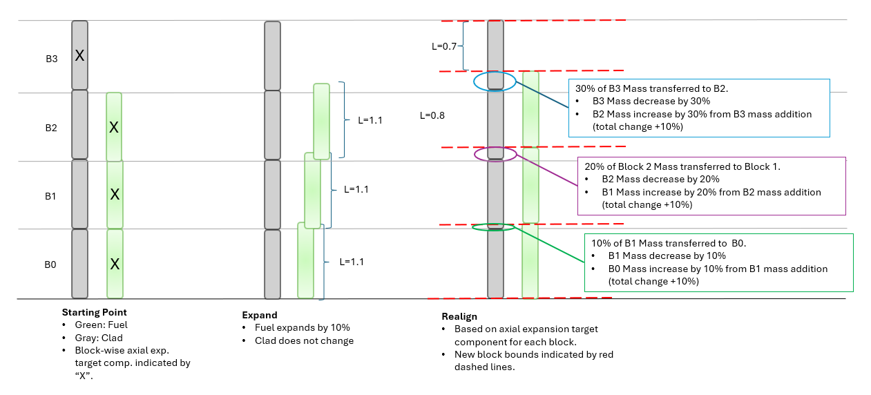
Illustration of mass redistribution for axial expansion in ARMI.

The redistribution process can be written mathematically. In Figure Illustration of mass redistribution for axial expansion in ARMI., consider the exchange of mass between the clad in Block 0 and Block 1,

(14)\[\hat{c}_{0,m} = c_{0,m} + 0.1c_{1,m}\]

(15)\[ \hat{c}_{1,m} = 0.9c_{1,m},\]

where \(c_{0/1,m}\) represents the clad mass in Block 0/1 prior to redistribution and \(\hat{c}_{0/1,m}\) represents the clad mass in Block 0/1 after redistribution, respectively. To compute the post-redistribution mass on-the-fly, the post-mass redistribution number densities, \(\hat{N}_{i,0/1}\), where the subscript \(i,0/1\) represents isotope \(i\) for Block 0/1, need to be computed.

Computing \(\hat{N}_{i,1}\) satisfying \(\hat{c}_{1,m}\) can be found by scaling the pre-redistribution number densities by the expansion factor. In practice however, the number densities are not changed and the mass is decreased through the reduction in the height of the parent Block.

Note

Recall, component mass in ARMI is calculated as the product of the mass density of the component, the area of the component, and the height of the block. The mass of components can be tuned through either of these three parameters.

Computing \(\hat{N}_{i,0}\) is non-trivial as, in general, \(c_0\) and \(c_1\) are at different temperatures. Consider,

(16)\[\begin{split}\hat{c}_{0,m} &= c_{0,m} + 0.1c_{1,m},\\ &= \sum_{x=0}^M N_{x,0} A_0(T_0) h_0 + 0.1 \sum_{j=0}^K N_{j,1} A_1(T_1) h_1,\\ \sum_{i=0}^P \hat{N}_{i,0} A_0(\hat{T}_0) \hat{h}_0 &= \sum_{x=0}^N N_{x,0} A_0(T_0) h_0 + \sum_{j=0}^K 0.1 N_{j,1} A_1(T_1) h_1 \big),\end{split}\]

where,

• \(A_{0/1}(T_{0/1})\) is the area of Component 0/1 at temperature 0/1,

• \(h_{0/1}\) is the height of Component 0/1,

• \(N\), \(K\) are the total number of isotopes in Component 0/1, respectively,

• \(P\) is the union of the isotopes in Component 0/1,

• and \(\hat{\square}\) represents post-redistribution values.

The post-redistribution height, \(\hat{h}_0\) is found to be the sum of the pre-expansion height, \(h_0\), and the different in z-elevation between it and the axial expansion target component for the Block, \(b\),

\[\begin{split}\hat{h}_0 &= h_0 + \delta,\\ &= h_0 + \left(b_{\text{ztop}} - c_{\text{ztop}}\right).\end{split}\]

Note

1. Recall, axial block bounds are determined by the axial expansion target component so the top z-elevation ztop for the block is the same as the top of the axial expansion target component.

2. In the axial expansion module, components are given z-elevation attributes. This information is not serialized to the database.

With \(\hat{h}_0\) known, the two remaining unknowns in Equation (16) are the post-redistribution temperature, \(\hat{T}_0\), and number densities, \(\hat{N}_{i,0}\). The latter are solved by using the expected post-redistribution per-isotope mass and component volume. The mass of isotope, \(i\), for Block 0/1 is calculated as follows,

\[m_{i,0/1} = N_{i,0/1} V_{0/1} \alpha_i \chi,\]

where \(\alpha_i\) is the atomic weight for isotope, \(i\), and \(\chi\) is a constant scaling from moles per cc to atoms per barn per cm. Given \(m_i\), the post redistribution number density is calculated as follows,

\[\hat{N}_{i,0} = \frac{\left( m_{i,0} + m_{i,1} \right) \chi}{ \big(A_1(T_1) h_1 + A_2(T_2)\delta\big) \alpha_i}.\]

The post redistribution temperature, \(\hat{T}_0\), is computed by minimizing the residual of the difference between the actual post-redistribution area of the Component and its expected area,

(17)\[\begin{split}A_0(\hat{T}_0) \left( h_1 + \delta \right) &= A_1(T_1) h_1 + A_2(T_2)\delta,\\ A_0(\hat{T}_0) &= \frac{A_1(T_1) h_1 + A_2(T_2)\delta}{h_1 + \delta}.\end{split}\]

The minimization of Equation (17) is solved using Brent’s method within scipy where the bounds of the solve are the temperatures of the two components exchanging mass, \(T_0\) and \(T_1\). In some instances, the minimization may fail. In this case, a mass weighted temperature is used instead,

(18)\[\hat{T}_0 = \frac{m_{i,0}T_0 + m_{i,1}T_1}{m_{i,0} + m_{i,1}}.\]

11.2.4. Warnings and Runtime Error Messages

11.2.4.1. Mass Redistribution Between Like Materials

Mass redistribution is currently only possible between components that are the same material. This restriction is to ensure that material properties post-redistribution are known (e.g., mixing different alloys of metal may result in a material with unknown properties). If components of different materials are attempted to have their mass redistributed, the following warning is populated to the stdout:

Cannot redistribute mass between components that are different materials!
  Trying to redistribute mass between the following components in <Assembly>:
      from --> {<Block 0>} : {<Component 0>} : {<Material 0>}
        to --> {<Block 1>} : {<Component 1>} : {<Material 1>}

  Instead, mass will be removed from (<Component 0> | <Material 0>) and
  (<Component 1> | <Material 1> will be artificially expanded. The consequence is that mass
  conservation is no longer guaranteed for the <Component 1> component type on this assembly!

11.2.4.2. Post-Redistribution Temperature Search Failure

As described in Section 11.2.3.1, the minimization of Equation (17) may fail. The two mechanisms in which Brent’s method may fail are if Equation (17) does not have opposite signs at each prescribed temperature bound of if Equation (17) is discontinuous. If the minimization routine fails, the following warning is printed to the stdout:

Temperature search algorithm in axial expansion has failed in <Assembly>
Trying to search for new temp between
    from --> <Block 0> : <Component 0> : <Material 0> at <Temperature 0> C
      to --> <Block 1> : <Component 1> : <Material 1> at <Temperature 1> C

f(<Temperature 0>) = {Area 0(Tc=<Temperature 0>) - targetArea}
f(<Temperature 1>) = {Area 0(Tc=<Temperature 1>) - targetArea}

Instead, a mass weighted average temperature of {Component 0} will be used. The consequence is that
mass conservation is no longer guaranteed for this component type on this assembly!

Note

The above warning has been limited to only components which have the FUEL or CONTROL flag. These are determined to be the most neutronically important components where the impact of this warning are the most relevant.

An example of where this warning may raise is in the following:

1. If two axially linked components have the same Thot values and different Tinput values, they will be the same temperature and have different areas. The range for the temperature search is null and will be impossible to find a temperature satisfying Equation (17).

2. If the coefficient of thermal expansion for a material is sufficiently small relative the difference in temperature between two component, the bounds of Equation (17) may not generate opposite signs and Brent’s method will fail.

11.2.4.3. Negative Block or Component Heights

If a Block or Component height becomes negative, an ArithmeticError is raised indicating which Block and/or Component has a negative height. Both signal a non-physical condition that is un-resolveable in the current implementation. This is often caused by thermal expansion of a solid component being drastically different that the other components nearby.

11.2.4.4. Inconsistent Component and Block Heights

The current implementation is designed such that the heights of each Component and their parent block remain consistent. However, these can go out of sync and have been found to be due incompatible blueprints definitions. As stated in Section 11.2.3, in order for mass to be conserved, each component must axially terminate in unique blocks. If a given blueprint does not meet this condition, the following warning may be raised for non-isothermal conditions:

The height of <Component> has gone out of sync with its parent block!
   Assembly: <Assembly>
      Block: <Block>
  Component: <Component>

      Block Height = <Block Height>
  Component Height = <Component Height>

The difference in height is <height difference> cm. This difference will result in an artificial
<"increase" or "decrease"> in the mass of <Component>. This is indicative that there are multiple axial component
terminations in <Block>. Per the ARMI User Manual, to preserve mass there can only be one axial component termination
per block.

If the different in height is positive, then the Component in question extends above the bounds of its parent Block and its mass will be artificially chopped proportional to the difference in height. If the difference in height is negative, the the Component in question stops below the bounds of the parent Block and its mass with artificially increase proportional to the different in height.

Note

The above warning has been limited to only components which have the FUEL or CONTROL flag. These are determined to be the most neutronically important components where the impact of this warning are the most relevant.